九、学习对象跟踪
在上一章中,我们学习了视频监控、背景建模和形态学图像处理。 我们讨论了如何使用不同的形态运算符将很酷的视觉效果应用到输入图像中。 在本章中,我们将学习如何跟踪实况视频中的对象。 我们将讨论可用于跟踪的对象的不同特征。 我们还将学习目标跟踪的不同方法和技术。 目标跟踪广泛应用于机器人、自动驾驶汽车、车辆跟踪、运动中的运动员跟踪和视频压缩。
在本章结束时,您将了解以下内容:
- 如何跟踪特定颜色的对象
- 如何构建交互式对象跟踪器
- 什么是拐角探测器?
- 如何检测要跟踪的好特征
- 如何构建基于光流的特征跟踪器
技术要求
本章要求熟悉 C++ 编程语言的基础知识。 本章中使用的所有代码都可以从以下 gihub 链接下载:https://github.com/PacktPublishing/Building-Computer-Vision-Projects-with-OpenCV4-and-CPlusPlus/tree/master/Chapter09。这些代码可以在任何操作系统上执行,尽管它只在 Ubuntu 上测试过。
请查看以下视频,了解实际操作中的代码: http://bit.ly/2SidbMc
跟踪特定颜色的对象
为了建立一个好的目标跟踪器,我们需要了解哪些特征可以用来使我们的跟踪健壮和准确。 所以,让我们朝这个方向迈出一小步,看看我们是否能利用色彩空间信息来设计出一个好的视觉跟踪器。 要记住的一件事是,颜色信息对照明条件很敏感。 在真实的应用中,您必须进行一些预处理来处理这些问题。 但现在,让我们假设其他人正在做这件事,我们得到的是清晰的彩色图像。
有许多不同的色彩空间,选择一个好的色彩空间将取决于用户使用的不同应用。 虽然 RGB 是计算机屏幕上的原生表示形式,但它对人类来说不一定是理想的。 当涉及到人类时,我们根据颜色的色调更自然地给颜色命名,这就是为什么色调饱和值(HSV)可能是信息最丰富的颜色空间之一。 它与我们感知颜色的方式密切相关。 色调指的是光谱,饱和度指的是特定颜色的强度,值指的是该像素的亮度。 这实际上是用柱面格式表示的。 你可以在http://infohost.nmt.edu/tcc/help/pubs/colortheory/web/hsv.html找到一个简单的解释。 我们可以将图像的像素放到 HSV 颜色空间中,然后使用该颜色空间来测量在该颜色空间中的距离和在该空间中的阈值,以跟踪给定的对象。
请考虑视频中的以下帧:
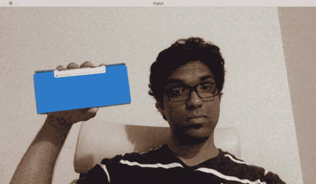
如果通过颜色空间滤镜运行它并跟踪该对象,您将看到如下所示:
正如我们在这里看到的,我们的跟踪器根据颜色特征识别视频中的特定对象。 为了使用这个跟踪器,我们需要知道目标对象的颜色分布。 下面是跟踪彩色对象的代码,它只选择具有特定给定色调的像素。 代码有很好的注释,因此请阅读每个术语的解释以了解发生了什么:
int main(int argc, char* argv[])
{
   // Variable declarations and initializations

    // Iterate until the user presses the Esc key
    while(true)
    {
        // Initialize the output image before each iteration
        outputImage = Scalar(0,0,0);

        // Capture the current frame
        cap >> frame;

        // Check if 'frame' is empty
        if(frame.empty())
            break;

        // Resize the frame
        resize(frame, frame, Size(), scalingFactor, scalingFactor, INTER_AREA);

        // Convert to HSV colorspace
        cvtColor(frame, hsvImage, COLOR_BGR2HSV);

        // Define the range of "blue" color in HSV colorspace
        Scalar lowerLimit = Scalar(60,100,100);
        Scalar upperLimit = Scalar(180,255,255);

        // Threshold the HSV image to get only blue color
        inRange(hsvImage, lowerLimit, upperLimit, mask);

        // Compute bitwise-AND of input image and mask
        bitwise_and(frame, frame, outputImage, mask=mask);

        // Run median filter on the output to smoothen it
        medianBlur(outputImage, outputImage, 5);

        // Display the input and output image
        imshow("Input", frame);
        imshow("Output", outputImage);

        // Get the keyboard input and check if it's 'Esc'
        // 30 -> wait for 30 ms
        // 27 -> ASCII value of 'ESC' key
        ch = waitKey(30);
        if (ch == 27) {
            break;
        }
    }

    return 1;
}
构建交互式对象跟踪器
基于颜色空间的跟踪器让我们可以自由地跟踪彩色对象,但我们也受到预定义颜色的限制。 如果我们只是想随机挑选一个对象呢? 我们如何构建一个能够学习所选对象的特征并自动跟踪它的对象跟踪器? 这就是c连续自适应 Mean Shift(CAMShift)算法出现的地方。 它基本上是均值漂移算法的改进版本。
均值漂移的概念实际上很好很简单。 假设我们选择了一个感兴趣的区域,并希望我们的对象跟踪器跟踪该对象。 在该区域中,我们根据颜色直方图选取一组点,并计算空间点的质心。 如果质心位于该区域的中心,我们就知道该物体没有移动。 但是如果质心不在这个区域的中心,那么我们就知道物体在朝某个方向移动。 质心的移动控制对象移动的方向。 因此,我们将对象的边界框移动到一个新位置,以便新的质心成为该边界框的中心。 因此,这种算法被称为均值移位,因为均值(质心)在移动。 这样,我们就可以随时了解对象的当前位置。
但是 Mean Shift 的问题是边界框的大小不允许改变。 当您将对象从相机移开时,该对象在人眼看来会变小,但 Mean Shift 不会考虑这一点。 在整个跟踪会话中,边界框的大小将保持不变。 因此,我们需要使用 CAMShift。 CAMShift 的优点是它可以根据对象的大小调整边界框的大小。 除此之外,它还可以跟踪物体的方位。
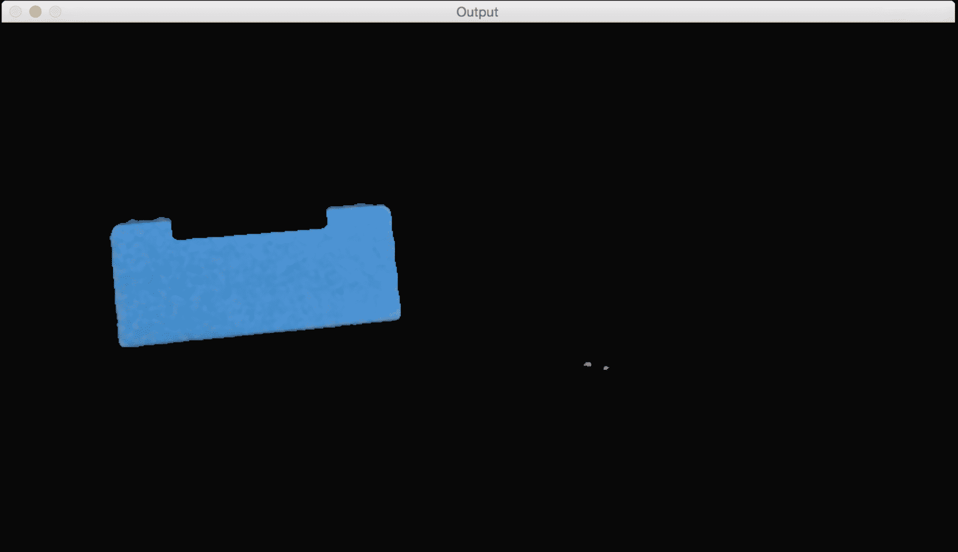
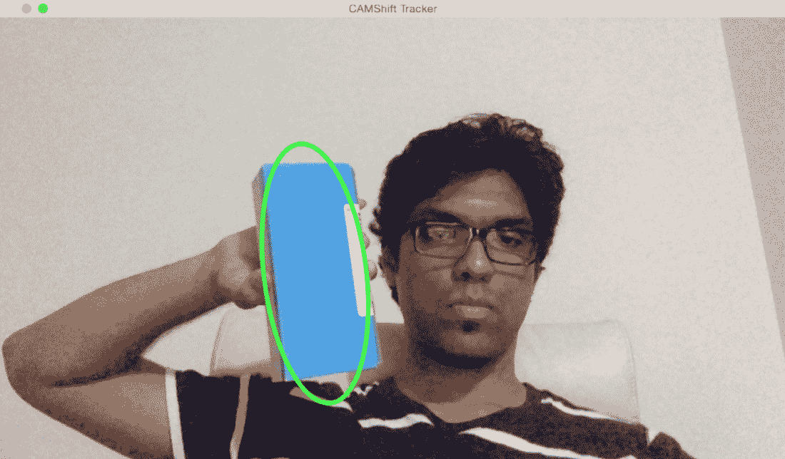
让我们考虑下面的帧,其中对象被高亮显示:
现在我们已经选择了对象,该算法计算直方图反投影并提取所有信息。 什么是直方图反投影? 这只是一种识别图像是否符合我们直方图模型的方法。 我们计算特定物体的直方图模型,然后使用该模型在图像中找到该物体。 让我们移动对象,看看它是如何被跟踪的:
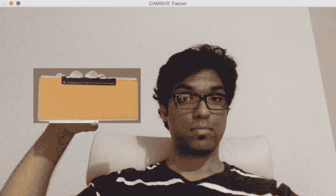
看起来这个物体被追踪得相当好。 让我们更改方向,看看追踪是否保持不变:
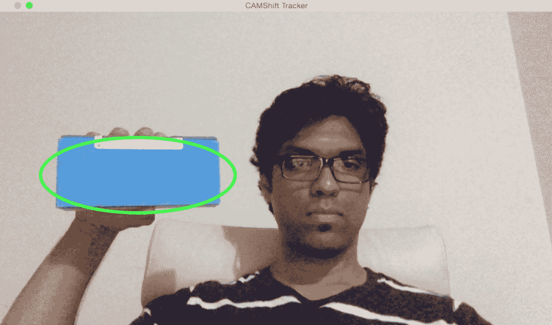
正如我们所看到的,边界椭圆已经改变了它的位置和方向。 让我们改变对象的视角,看看它是否仍然能够跟踪它:
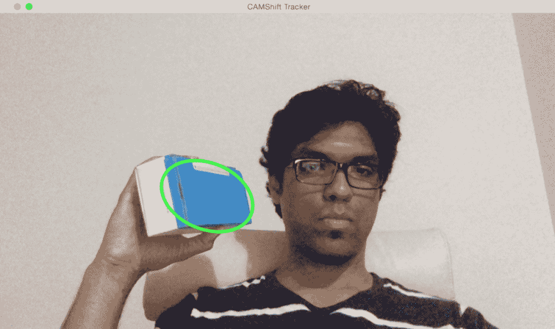
我们还是很棒的! 边界椭圆更改了纵横比,以反映对象现在看起来倾斜的事实(因为透视变换)。 让我们看看代码中的用户界面功能:
Mat image;
Point originPoint;
Rect selectedRect;
bool selectRegion = false;
int trackingFlag = 0;

// Function to track the mouse events
void onMouse(int event, int x, int y, int, void*)
{
    if(selectRegion)
    {
        selectedRect.x = MIN(x, originPoint.x);
        selectedRect.y = MIN(y, originPoint.y);
        selectedRect.width = std::abs(x - originPoint.x);
        selectedRect.height = std::abs(y - originPoint.y);

        selectedRect &= Rect(0, 0, image.cols, image.rows);
    }

    switch(event)
    {
        case EVENT_LBUTTONDOWN:
            originPoint = Point(x,y);
            selectedRect = Rect(x,y,0,0);
            selectRegion = true;
            break;

        case EVENT_LBUTTONUP:
            selectRegion = false;
            if( selectedRect.width > 0 && selectedRect.height > 0 )
            {
                trackingFlag = -1;
            }
            break;
    }
}
此函数基本上捕获在窗口中选择的矩形的坐标。 用户只需用鼠标点击并拖动即可。 OpenCV 中有一组内置函数可以帮助我们检测这些不同的鼠标事件。
以下是基于 CAMShift 执行对象跟踪的代码:
int main(int argc, char* argv[])
{
    // Variable declaration and initialization
    ....
    // Iterate until the user presses the Esc key
    while(true)
    {
        // Capture the current frame
        cap >> frame;

        // Check if 'frame' is empty
        if(frame.empty())
            break;

        // Resize the frame
        resize(frame, frame, Size(), scalingFactor, scalingFactor, INTER_AREA);

        // Clone the input frame
        frame.copyTo(image);

        // Convert to HSV colorspace
        cvtColor(image, hsvImage, COLOR_BGR2HSV);
现在我们有了 HSV 图像等待处理。 让我们继续看看如何使用我们的阈值来处理此图像:
        if(trackingFlag)
        {
            // Check for all the values in 'hsvimage' that are within the specified range
            // and put the result in 'mask'
            inRange(hsvImage, Scalar(0, minSaturation, minValue), Scalar(180, 256, maxValue), mask);

            // Mix the specified channels
            int channels[] = {0, 0};
            hueImage.create(hsvImage.size(), hsvImage.depth());
            mixChannels(&hsvImage, 1, &hueImage, 1, channels, 1);

            if(trackingFlag < 0)
            {
                // Create images based on selected regions of interest
                Mat roi(hueImage, selectedRect), maskroi(mask, selectedRect);

                // Compute the histogram and normalize it
                calcHist(&roi, 1, 0, maskroi, hist, 1, &histSize, &histRanges);
                normalize(hist, hist, 0, 255, NORM_MINMAX);

                trackingRect = selectedRect;
                trackingFlag = 1;
            }
正如我们在这里看到的,我们使用 HSV 图像来计算区域的直方图。 我们使用我们的阈值在 HSV 谱中定位所需的颜色,然后在此基础上过滤掉图像。 让我们继续看看如何计算直方图反投影:
            // Compute the histogram backprojection
            calcBackProject(&hueImage, 1, 0, hist, backproj, &histRanges);
            backproj &= mask;
            RotatedRect rotatedTrackingRect = CamShift(backproj, trackingRect, TermCriteria(TermCriteria::EPS | TermCriteria::COUNT, 10, 1));

            // Check if the area of trackingRect is too small
            if(trackingRect.area() <= 1)
            {
                // Use an offset value to make sure the trackingRect has a minimum size
                int cols = backproj.cols, rows = backproj.rows;
                int offset = MIN(rows, cols) + 1;
                trackingRect = Rect(trackingRect.x - offset, trackingRect.y - offset, trackingRect.x + offset, trackingRect.y + offset) & Rect(0, 0, cols, rows);
            }
现在我们准备好显示结果了。 使用旋转的矩形,让我们围绕感兴趣的区域绘制一个椭圆:
            // Draw the ellipse on top of the image
            ellipse(image, rotatedTrackingRect, Scalar(0,255,0), 3, LINE_AA);
        }

        // Apply the 'negative' effect on the selected region of interest
        if(selectRegion && selectedRect.width > 0 && selectedRect.height > 0)
        {
            Mat roi(image, selectedRect);
            bitwise_not(roi, roi);
        }

        // Display the output image
        imshow(windowName, image);

        // Get the keyboard input and check if it's 'Esc'
        // 27 -> ASCII value of 'Esc' key
        ch = waitKey(30);
        if (ch == 27) {
            break;
        }
    }

    return 1;
}
使用 Harris 角点检测器检测点
角点检测是一种用于检测图像中的兴趣点的技术。 这些兴趣点在计算机视觉术语中也称为特征点,或简称为特征。 拐角基本上是两条边的交集。 兴趣点基本上是可以在图像中唯一检测到的东西。 角是兴趣点的一种特殊情况。 这些兴趣点帮助我们描述图像的特征。 这些点在诸如目标跟踪、图像分类和视觉搜索等应用中被广泛使用。 既然我们知道角点很有趣,让我们看看如何检测它们。
在计算机视觉中,有一种流行的角点检测技术,称为 Harris 角点检测器。 我们基本上是基于灰度图像的偏导数构造一个 2x2 矩阵,然后对特征值进行分析。 这到底是什么意思? 好吧,让我们仔细分析一下,这样我们就能更好地理解它。 让我们考虑一下图像中的一个小补丁。 我们的目标是确定这个补丁中是否有角落。 因此,我们考虑所有的邻域面片,并计算我们的面片与所有邻域面片之间的亮度差。 如果各个方向的差异都很大,那么我们就知道我们的地块有一个角落。 这是对实际算法的过度简化,但它涵盖了要点。 如果你想了解基本的数学细节,你可以在http://www.bmva.org/bmvc/1988/avc-88-023.pdf查看Harris和Stephens的原文。 拐角是指沿两个方向的强度差异很大的点。
如果我们运行 Harris 角检测器,它将如下所示:
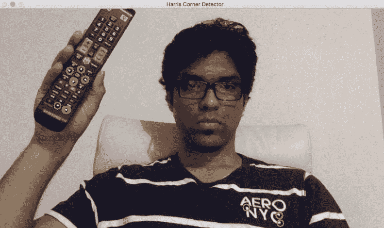
正如我们所看到的,电视遥控器上的绿色圆圈是检测到的角落。 这将根据您为检测器选择的参数进行更改。 如果修改参数,您可以看到可能会检测到更多的点。 如果您将其设置为严格,则可能无法检测到软角。 让我们看一下检测哈里斯拐角的代码:
int main(int argc, char* argv[])
{
// Variable declaration and initialization

// Iterate until the user presses the Esc key
while(true)
{
    // Capture the current frame
    cap >> frame;

    // Resize the frame
    resize(frame, frame, Size(), scalingFactor, scalingFactor, INTER_AREA);

    dst = Mat::zeros(frame.size(), CV_32FC1);

    // Convert to grayscale
    cvtColor(frame, frameGray, COLOR_BGR2GRAY );

    // Detecting corners
    cornerHarris(frameGray, dst, blockSize, apertureSize, k, BORDER_DEFAULT);

    // Normalizing
    normalize(dst, dst_norm, 0, 255, NORM_MINMAX, CV_32FC1, Mat());
    convertScaleAbs(dst_norm, dst_norm_scaled);
我们将图像转换为灰度图像,并使用参数检测角点。 您可以在.cpp文件中找到完整的代码。 这些参数在将要检测的点数中起着重要作用。 您可以在https://docs.opencv.org/master/dd/d1a/group__imgproc__feature.html#gac1fc3598018010880e370e2f709b4345查看cornerHarris()的 OpenCV 文档。
我们现在有了我们需要的所有信息。 让我们继续在我们的角落周围画圈,以显示结果:
        // Drawing a circle around each corner
        for(int j = 0; j < dst_norm.rows ; j++)
        {
            for(int i = 0; i < dst_norm.cols; i++)
            {
                if((int)dst_norm.at<float>(j,i) > thresh)
                {
                    circle(frame, Point(i, j), 8, Scalar(0,255,0), 2, 8, 0);
                }
            }
        }

        // Showing the result
        imshow(windowName, frame);

        // Get the keyboard input and check if it's 'Esc'
        // 27 -> ASCII value of 'Esc' key
        ch = waitKey(10);
        if (ch == 27) {
            break;
        }
    }

    // Release the video capture object
    cap.release();

    // Close all windows
    destroyAllWindows();

    return 1;
}
正如我们所看到的,这段代码接受一个输入参数:blockSize。 根据您选择的大小,性能会有所不同。 从值 4 开始,试着使用它,看看会发生什么。
要跟踪的良好功能
Harris 角点检测器在很多情况下都表现良好,但仍有改进的余地。 大约在Harris和Stephens、Shii和Tomasi最初的论文发表 6 年后,他们将其称为跟踪的良好特征。 你可以在这里阅读原文:http://www.ai.mit.edu/courses/6.891/handouts/shi94good.pdf。 他们使用了不同的评分函数来提高整体质量。 使用这种方法,我们可以在给定的图像中找到 N 个最强的角点。 当我们不想使用每个角落来从图像中提取信息时,这是非常有用的。 正如我们所讨论的,一个好的兴趣点检测器在目标跟踪、目标识别和图像搜索等应用中非常有用。
如果将 Shii-Tomasi 角点检测器应用于图像,您将看到如下所示:
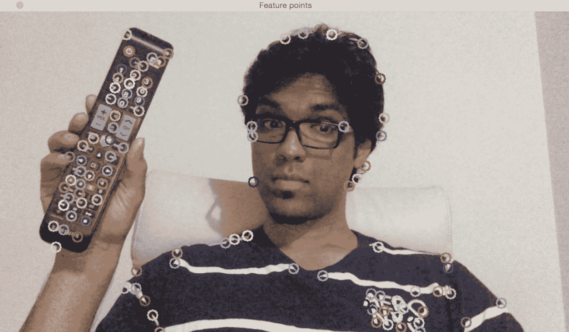
正如我们在这里看到的,帧中的所有重要点都被捕捉到了。 让我们看一下跟踪这些功能的代码:
int main(int argc, char* argv[])
{
    // Variable declaration and initialization

    // Iterate until the user presses the Esc key
    while(true)
    {
        // Capture the current frame
        cap >> frame;

        // Resize the frame
        resize(frame, frame, Size(), scalingFactor, scalingFactor, INTER_AREA);

        // Convert to grayscale
        cvtColor(frame, frameGray, COLOR_BGR2GRAY );

        // Initialize the parameters for Shi-Tomasi algorithm
        vector<Point2f> corners;
        double qualityThreshold = 0.02;
        double minDist = 15;
        int blockSize = 5;
        bool useHarrisDetector = false;
        double k = 0.07;

        // Clone the input frame
        Mat frameCopy;
        frameCopy = frame.clone();

        // Apply corner detection
        goodFeaturesToTrack(frameGray, corners, numCorners, qualityThreshold, minDist, Mat(), blockSize, useHarrisDetector, k);
正如我们所看到的,我们提取了帧,并使用goodFeaturesToTrack来检测角点。 重要的是要理解,检测到的角点数量将取决于我们选择的参数。 你可以在http://docs.opencv.org/2.4/modules/imgproc/doc/feature_detection.html?highlight=goodfeaturestotrack#goodfeaturestotrack上找到详细的解释。 让我们继续在这些点上画圆圈以显示输出图像:
        // Parameters for the circles to display the corners
        int radius = 8;      // radius of the circles
        int thickness = 2;   // thickness of the circles
        int lineType = 8;

        // Draw the detected corners using circles
        for(size_t i = 0; i < corners.size(); i++)
        {
            Scalar color = Scalar(rng.uniform(0,255), rng.uniform(0,255), rng.uniform(0,255));
            circle(frameCopy, corners[i], radius, color, thickness, lineType, 0);
        }

        /// Show what you got
        imshow(windowName, frameCopy);

        // Get the keyboard input and check if it's 'Esc'
        // 27 -> ASCII value of 'Esc' key
        ch = waitKey(30);
        if (ch == 27) {
            break;
        }
    }

    // Release the video capture object
    cap.release();

    // Close all windows
    destroyAllWindows();

    return 1;
}
该程序接受一个输入参数:numCorners。 该值指示要跟踪的最大角点数。 从值100开始,试着使用它,看看会发生什么。 如果增加此值,您将看到检测到更多的特征点。
基于特征的跟踪
基于特征的跟踪是指在视频中的连续帧上跟踪单个特征点。 这里的优点是我们不必在每一帧中都检测特征点。 我们只能探测到他们一次,然后继续追踪他们。 这比在每一帧上运行检测器效率更高。 我们使用一种叫做光流的技术来跟踪这些特征。 光流是计算机视觉中最流行的技术之一。 我们选择一组特征点,并通过视频流跟踪它们。 当我们检测特征点时,我们计算位移向量,并显示这些关键点在连续帧之间的运动。 这些矢量称为运动矢量。 与前一帧相比,特定点的运动矢量基本上只是一条指示该点移动位置的方向线。 使用不同的方法来检测这些运动矢量。 最流行的两个算法是Lucas-Kanade方法和Farneback算法。
卢卡斯-卡纳德法
稀疏光流跟踪采用 Lucas-Kanade 方法。 我们所说的稀疏是指特征点的数量相对较少。 您可以在这里参考他们的原文:http://cseweb.ucsd.edu/classes/sp02/cse252/lucaskanade81.pdf。 我们从提取特征点开始这个过程。 对于每个特征点,我们以特征点为中心创建 3 x 3 面片。 这里的假设是,每个面片中的所有点都会有类似的运动。 我们可以根据手头的问题调整此窗口的大小。
对于当前帧中的每个特征点,我们将周围的 3x3 面片作为参考点。 对于此补丁,我们在前一帧的邻域中查找,以获得最佳匹配。 这个邻域通常大于 3x3,因为我们希望得到最接近所考虑的面片的面片。 现在,从上一帧中匹配面片的中心像素到当前帧中正在考虑的面片的中心像素的路径将成为运动向量。 我们对所有的特征点都这样做,并提取所有的运动矢量。
让我们考虑以下框架:
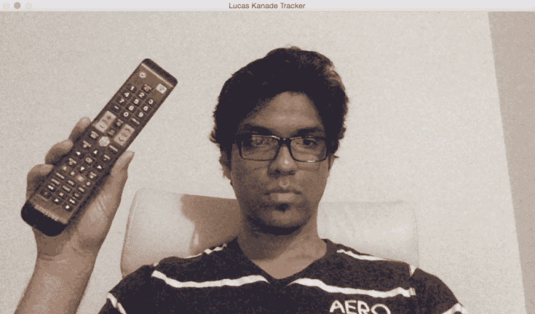
我们需要添加一些我们想要跟踪的点。 只需用鼠标单击此窗口上的一系列点即可:
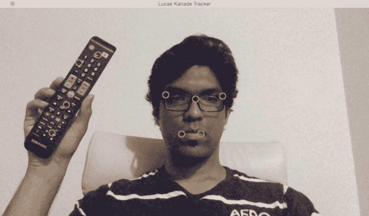
如果我移动到不同的位置,您将看到这些点仍在一个小误差范围内被正确跟踪:
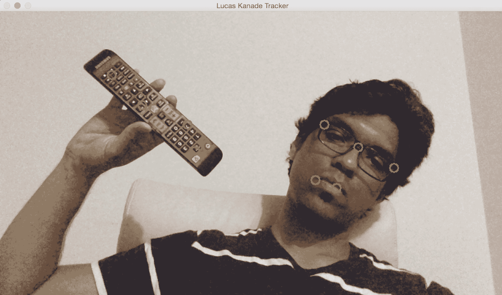
让我们加很多分,看看会发生什么:
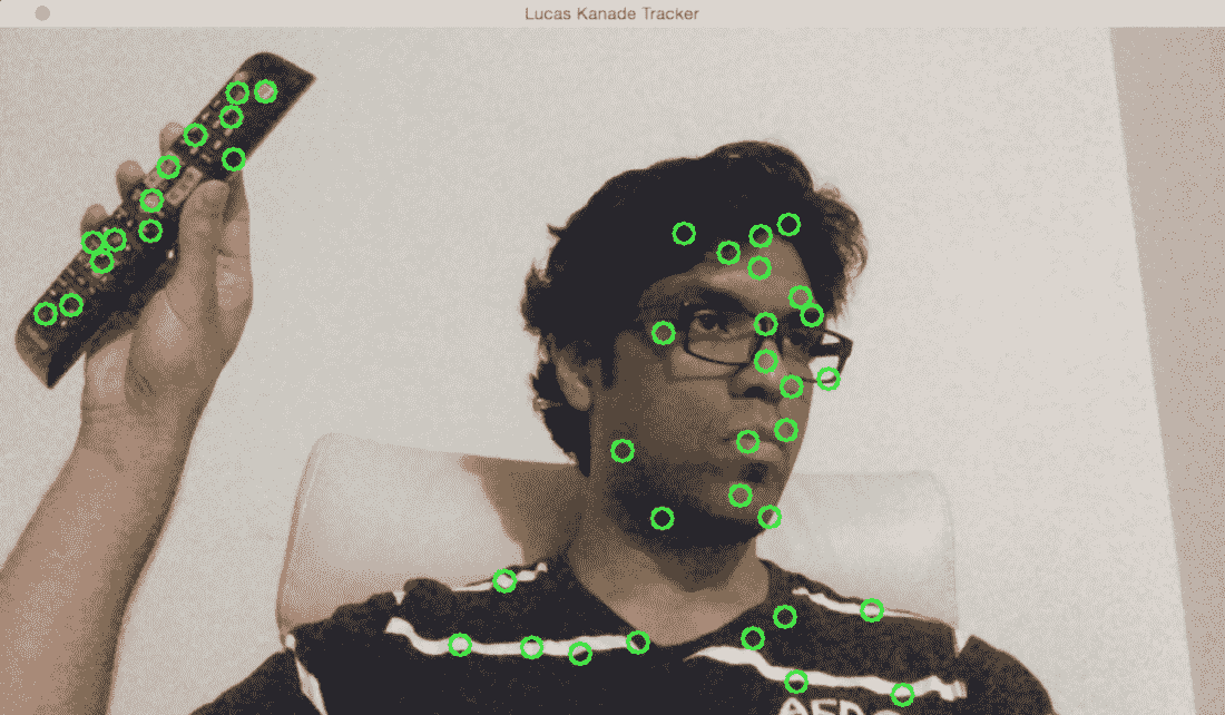
正如我们所看到的,它将继续跟踪这些点。 但是,你会注意到,一些点会因为突出程度或移动速度等因素而丢失。 如果你想玩这个游戏,你可以继续给它加更多的分数。 您还可以让用户在输入视频中选择感兴趣的区域。 然后,可以从该感兴趣区域提取特征点,并通过绘制边界框追踪对象。 这将是一次有趣的练习!
以下是执行基于 Lucas-Kanade 的跟踪的代码:
int main(int argc, char* argv[])
{
    // Variable declaration and initialization

    // Iterate until the user hits the Esc key
    while(true)
    {
        // Capture the current frame
        cap >> frame;

        // Check if the frame is empty
        if(frame.empty())
            break;

        // Resize the frame
        resize(frame, frame, Size(), scalingFactor, scalingFactor, INTER_AREA);

        // Copy the input frame
        frame.copyTo(image);

        // Convert the image to grayscale
        cvtColor(image, curGrayImage, COLOR_BGR2GRAY);

        // Check if there are points to track
        if(!trackingPoints[0].empty())
        {
            // Status vector to indicate whether the flow for the corresponding features has been found
            vector<uchar> statusVector;

            // Error vector to indicate the error for the corresponding feature
            vector<float> errorVector;

            // Check if previous image is empty
            if(prevGrayImage.empty())
            {
                curGrayImage.copyTo(prevGrayImage);
            }

            // Calculate the optical flow using Lucas-Kanade algorithm
            calcOpticalFlowPyrLK(prevGrayImage, curGrayImage, trackingPoints[0], trackingPoints[1], statusVector, errorVector, windowSize, 3, terminationCriteria, 0, 0.001);
我们使用当前图像和前一图像来计算光流信息。 不用说,输出的质量将取决于所选择的参数。 有关参数的更多详细信息,请访问http://docs.opencv.org/2.4/modules/video/doc/motion_analysis_and_object_tracking.html#calcopticalflowpyrlk。 为了提高质量和健壮性,我们需要过滤掉彼此非常接近的点,因为它们不会添加新的信息。 让我们继续这样做:
            int count = 0;

            // Minimum distance between any two tracking points
            int minDist = 7;

            for(int i=0; i < trackingPoints[1].size(); i++)
            {
                if(pointTrackingFlag)
                {
                    // If the new point is within 'minDist' distance from an existing point, it will not be tracked
                    if(norm(currentPoint - trackingPoints[1][i]) <= minDist)
                    {
                        pointTrackingFlag = false;
                        continue;
                    }
                }

                // Check if the status vector is good
                if(!statusVector[i])
                    continue;

                trackingPoints[1][count++ ] = trackingPoints[1][i];

                // Draw a filled circle for each of the tracking points
                int radius = 8;
                int thickness = 2;
                int lineType = 8;
                circle(image, trackingPoints[1][i], radius, Scalar(0,255,0), thickness, lineType);
            }

            trackingPoints[1].resize(count);
        }
我们现在有了跟踪点。 下一步是细化这些点的位置。 在这种情况下,Refined的确切含义是什么? 为了提高计算速度,需要进行一定程度的量化。 用外行的话说,你可以把它看作是四舍五入。 现在我们有了大致的区域,我们可以细化该区域内点的位置,以获得更准确的结果。 让我们继续这样做:
        // Refining the location of the feature points
        if(pointTrackingFlag && trackingPoints[1].size() < maxNumPoints)
        {
            vector<Point2f> tempPoints;
            tempPoints.push_back(currentPoint);

            // Function to refine the location of the corners to subpixel accuracy.
            // Here, 'pixel' refers to the image patch of size 'windowSize' and not the actual image pixel
            cornerSubPix(curGrayImage, tempPoints, windowSize, Size(-1,-1), terminationCriteria);

            trackingPoints[1].push_back(tempPoints[0]);
            pointTrackingFlag = false;
        }

        // Display the image with the tracking points
        imshow(windowName, image);

        // Check if the user pressed the Esc key
        char ch = waitKey(10);
        if(ch == 27)
            break;

        // Swap the 'points' vectors to update 'previous' to 'current'
        std::swap(trackingPoints[1], trackingPoints[0]);

        // Swap the images to update previous image to current image
        cv::swap(prevGrayImage, curGrayImage);
    }

    return 1;
}
Farneback 算法
冈纳·法内巴克(Gunnar Farneback)提出了这种光流算法,用于密集跟踪。 密集跟踪在机器人、增强现实和 3D 地图中被广泛使用。 您可以在这里查看原文:http://www.diva-portal.org/smash/get/diva2:273847/FULLTEXT01.pdf。 Lucas-Kanade 方法是一种稀疏技术,这意味着我们只需要处理整个图像中的一些像素。 另一方面,Farneback 算法是一种密集技术,需要我们处理给定图像中的所有像素。 因此,很明显,这是一种权衡。 密集技术更精确,但速度更慢。 稀疏技术的精确度较低,但速度更快。 对于实时应用,人们倾向于使用稀疏技术。 对于时间和复杂性不是一个因素的应用,人们倾向于使用密集技术来提取更精细的细节。
在他的论文中,Farneback 描述了一种基于多项式展开的两帧密集光流估计方法。 我们的目标是估计这两个帧之间的运动,这基本上是一个分三步走的过程。 在第一步中,用多项式逼近两帧中的每个邻域。 在这种情况下,我们只对二次多项式感兴趣。 下一步是通过全局位移构造新的信号。 现在每个邻域都用一个多项式来近似,我们需要看看如果这个多项式经过理想的平移会发生什么。 最后一步是通过将这些二次多项式的产量中的系数相等来计算全局位移。
现在,这怎么可能呢? 如果你仔细想想,我们假设一个完整的信号是一个单一的多项式,并且这两个信号之间存在全局平移。 这不是一个现实的场景! 那么,我们在找什么呢? 嗯,我们的目标是找出这些误差是否足够小,这样我们就可以建立一个有用的算法来跟踪这些特征。
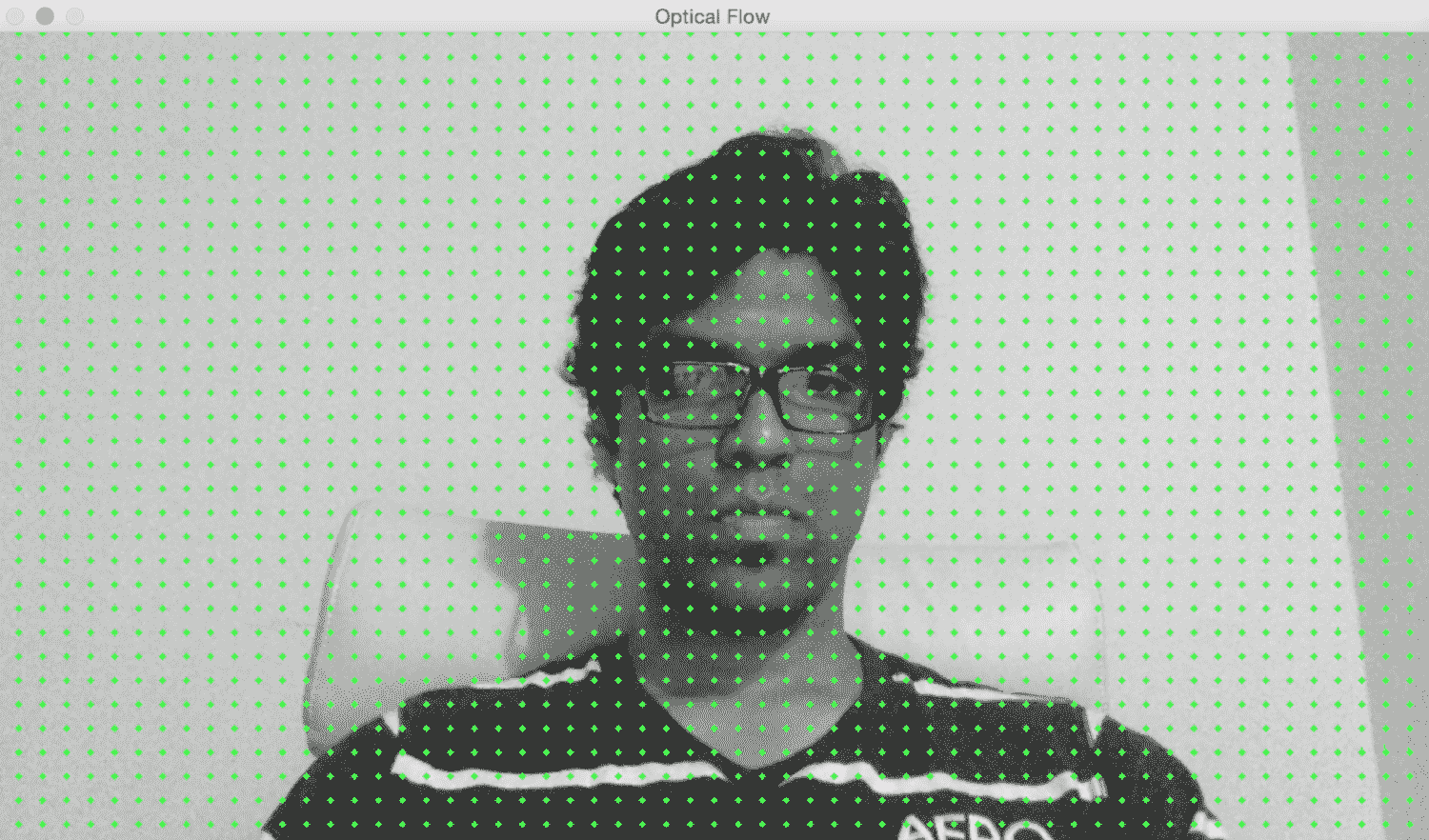
让我们看一张静态图像:
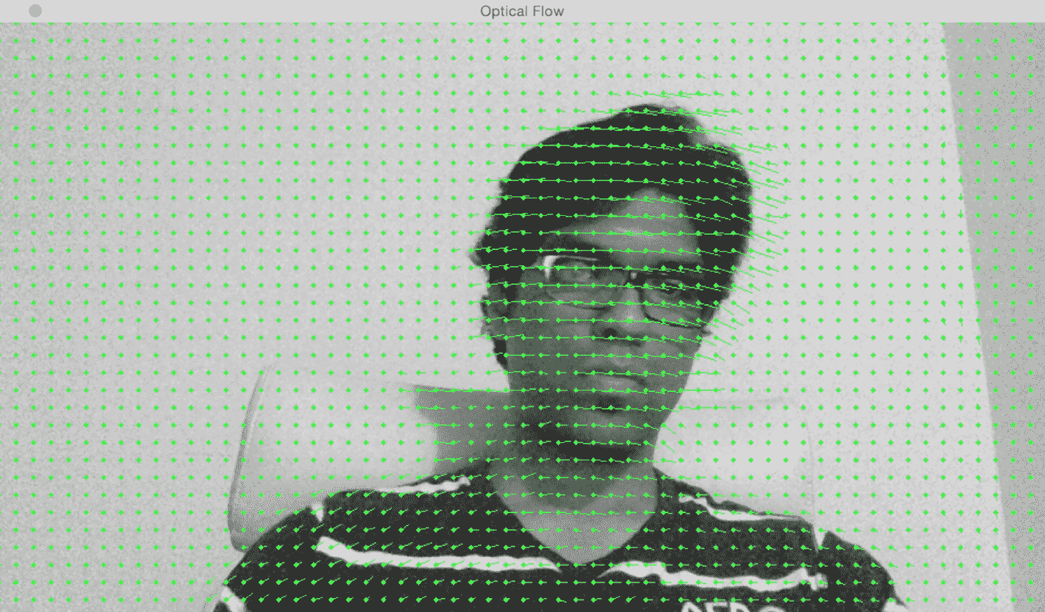
如果我横向移动,我们可以看到运动矢量指向水平方向。 它只是简单地跟踪我的头部运动:
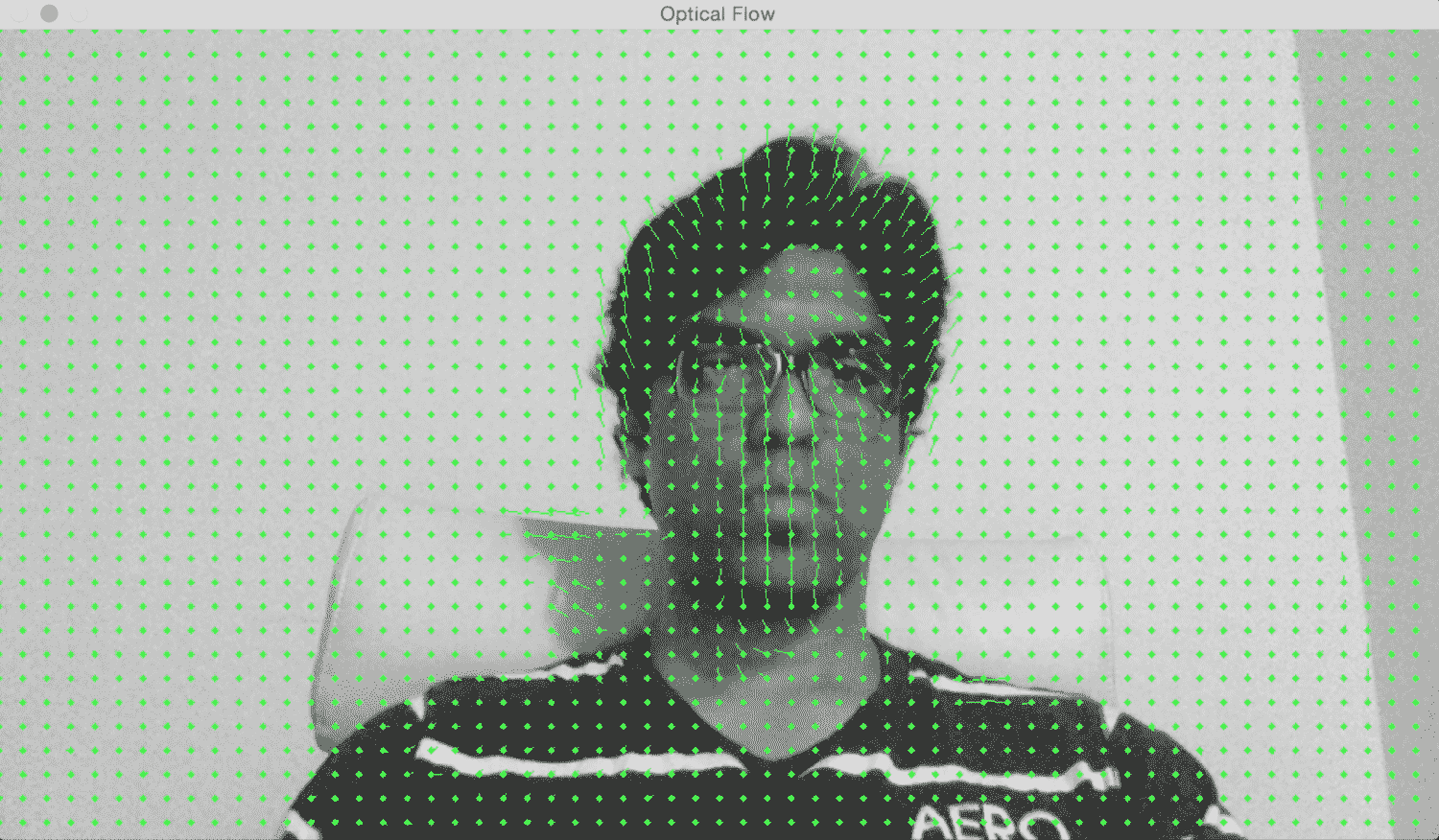
如果我离开网络摄像头,您可以看到运动矢量指向垂直于图像平面的方向:
以下是使用 Farneback 算法进行基于光流的跟踪的代码:
int main(int, char** argv)
{
    // Variable declaration and initialization

    // Iterate until the user presses the Esc key
    while(true)
    {
        // Capture the current frame
        cap >> frame;

        if(frame.empty())
            break;

        // Resize the frame
        resize(frame, frame, Size(), scalingFactor, scalingFactor, INTER_AREA);

        // Convert to grayscale
        cvtColor(frame, curGray, COLOR_BGR2GRAY);

        // Check if the image is valid
        if(prevGray.data)
        {
            // Initialize parameters for the optical flow algorithm
            float pyrScale = 0.5;
            int numLevels = 3;
            int windowSize = 15;
            int numIterations = 3;
            int neighborhoodSize = 5;
            float stdDeviation = 1.2;

            // Calculate optical flow map using Farneback algorithm
            calcOpticalFlowFarneback(prevGray, curGray, flowImage, pyrScale, numLevels, windowSize, numIterations, neighborhoodSize, stdDeviation, OPTFLOW_USE_INITIAL_FLOW);
正如我们所看到的,我们使用 Farneback 算法来计算光流矢量。 当涉及到跟踪质量时,calcOpticalFlowFarneback的输入参数很重要。 您可以在http://docs.opencv.org/3.0-beta/modules/video/doc/motion_analysis_and_object_tracking.html上找到有关这些参数的详细信息。 让我们继续在输出图像上绘制这些向量:
            // Convert to 3-channel RGB
            cvtColor(prevGray, flowImageGray, COLOR_GRAY2BGR);

            // Draw the optical flow map
            drawOpticalFlow(flowImage, flowImageGray);

            // Display the output image
            imshow(windowName, flowImageGray);
        }

        // Break out of the loop if the user presses the Esc key
        ch = waitKey(10);
        if(ch == 27)
            break;

        // Swap previous image with the current image
        std::swap(prevGray, curGray);
    }

    return 1;
}
我们使用一个名为drawOpticalFlow的函数来绘制这些光流矢量。 这些矢量表示运动的方向。 让我们看一下该函数,看看我们是如何绘制这些向量的:
// Function to compute the optical flow map
void drawOpticalFlow(const Mat& flowImage, Mat& flowImageGray)
{
    int stepSize = 16;
    Scalar color = Scalar(0, 255, 0);

    // Draw the uniform grid of points on the input image along with the motion vectors
    for(int y = 0; y < flowImageGray.rows; y += stepSize)
    {
        for(int x = 0; x < flowImageGray.cols; x += stepSize)
        {
            // Circles to indicate the uniform grid of points
            int radius = 2;
            int thickness = -1;
            circle(flowImageGray, Point(x,y), radius, color, thickness);

            // Lines to indicate the motion vectors
            Point2f pt = flowImage.at<Point2f>(y, x);
            line(flowImageGray, Point(x,y), Point(cvRound(x+pt.x), cvRound(y+pt.y)), color);
        }
    }
}
简略的 / 概括的 / 简易判罪的 / 简易的
在本章中,我们学习了目标跟踪。 我们学习了如何使用 HSV 色彩空间来跟踪特定颜色的对象。 我们讨论了用于对象跟踪的群集技术,以及如何使用 CAMShift 算法构建交互式对象跟踪器。 我们研究了角点探测器,以及如何在现场视频中跟踪角点。 我们讨论了如何使用光流跟踪视频中的特征。 最后,我们理解了 Lucas-Kanade 和 Farneback 算法背后的概念,然后实现了它们。
在下一章中,我们将讨论分割算法以及如何将其用于文本识别。
